


Data Structures Explained: Arrays, Linked Lists, Trees & Graphs
⚡ Quick Answer
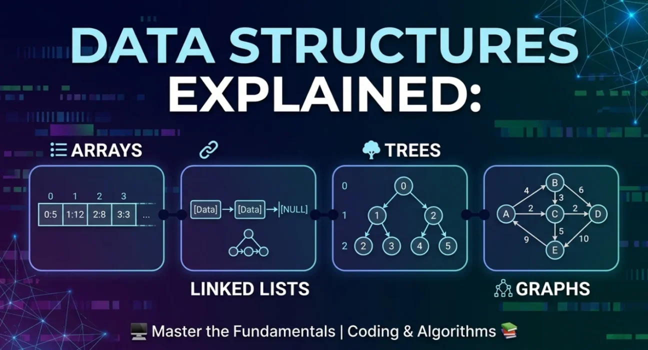
A data structure organises and stores data in memory for efficient access and modification. The four core types are Arrays (contiguous indexed storage), Linked Lists (dynamic node chains), Trees (hierarchical parent-child structures), and Graphs (networks of nodes and edges). Each has unique trade-offs in speed, memory, and use case.
Introduction: Why Data Structures Matter
Imagine trying to find a book in a library where every book is scattered randomly on the floor. Finding your book would take forever. But if the library organises books by genre, author, and title — your search becomes instant.
That is precisely what data structures do for your programs. They organise data so it can be accessed, processed, and stored as efficiently as possible. Whether you are building a calculator or a large-scale platform like Facebook, your choice of data structure directly affects speed, memory usage, and overall performance.
In this tutorial, you will learn the four most important data structures every programmer must know — with real code, complexity analysis, and the real-world contexts where each shines.
1. Arrays: The Foundation of All Data Structures
What is an Array?
An array is the simplest and most widely used data structure. It stores a collection of elements in contiguous (adjacent) memory locations, where each element is identified by a zero-based index.
Think of an array as a row of numbered mailboxes. Each mailbox has a unique number (its index), and you can go directly to any mailbox if you know its number. This is why arrays support random access — retrieving any element takes the same time regardless of array size.
How Arrays Work in Memory
When you declare an array, the program reserves a fixed block of contiguous memory. Because every element occupies the same space, the exact address of any element can be calculated instantly:
C++ — Array Memory Access
// Address formula
Address of arr[i] = Base Address + (i × element size)

int arr[5] = {10, 20, 30, 40, 50};
// arr[0] → 10  (O(1) access)
// arr[2] → 30  (O(1) access)
// arr[4] → 50  (O(1) access)
Time & Space Complexity
| Operation | Complexity | Why |
|---|---|---|
| Access by index | O(1) | Direct calculation via base address |
| Search (unsorted) | O(n) | Check each element one by one |
| Search (sorted, binary) | O(log n) | Divide and conquer |
| Insert at beginning | O(n) | All elements must shift right |
| Insert at end | O(1) | No shifting needed |
| Delete element | O(n) | Elements must shift to fill gap |
| Space | O(n) | n slots occupy n memory locations |
Real-World Applications
- Image processing — a digital image is a 2D array of pixel values
- Spreadsheets — Excel cells are stored as a 2D array of rows and columns
- Machine learning — tensors (multi-dimensional arrays) power neural networks
- Hash tables — arrays are the underlying structure of most hash maps
✓ When to Use Arrays
Use arrays when you know the size in advance, need fast random access by index, and work with homogeneous data. Avoid them when you need frequent mid-array insertions/deletions or when the data size changes dynamically.
2. Linked Lists: Dynamic and Flexible Storage
What is a Linked List?
Unlike arrays, a linked list does not store elements in contiguous memory. Instead, it is made up of nodes, where each node contains the actual data and a pointer to the next node in the sequence.
A good analogy is a treasure hunt. Each clue (node) contains a piece of treasure (data) and a hint about where to find the next clue (pointer). You cannot skip directly to clue 5 — you must follow the chain from the beginning. This is why linked lists do not support direct random access.
C++ — Linked List Node
struct Node {
    int   data;   // The actual value
    Node* next;   // Pointer to next node
};

// Building: 10 → 20 → 30 → NULL
Node* head = new Node{10, nullptr};
head->next          = new Node{20, nullptr};
head->next->next    = new Node{30, nullptr};
Types of Linked Lists
- Singly Linked List — each node points only to the next; traversal in one direction only
- Doubly Linked List — each node has both a next and a previous pointer, enabling bidirectional traversal
- Circular Linked List — the last node points back to the first, forming a loop; used in round-robin scheduling
Arrays vs Linked Lists at a Glance
| Factor | Array | Linked List |
|---|---|---|
| Memory allocation | Static (fixed at creation) | Dynamic (grows/shrinks at runtime) |
| Access speed | O(1) — random access | O(n) — sequential only |
| Insert / Delete | O(n) — shifting required | O(1) at a known position |
| Memory overhead | Less — no pointers | More — stores data + pointer |
| Cache performance | Excellent (contiguous) | Poor (scattered in memory) |
| Best use case | Known size, frequent reads | Frequent inserts/deletes |
Real-World Applications
- Browser history — forward/back navigation uses a doubly linked list
- Music players — previous/next track is a classic doubly linked list operation
- Undo/redo — text editors store states as a linked list of history snapshots
- Memory allocation — operating systems track free memory blocks using linked lists
⚠ When to Use Linked Lists
Use linked lists when data size is unknown or changes frequently, and when you need efficient insertions or deletions at the head or tail. Avoid them when you need fast random access or when memory is tightly constrained.
3. Trees: Hierarchical Structures for Organised Data
What is a Tree?
Up to this point, we have examined linear structures. Now it is time to move into non-linear territory. A tree is a hierarchical data structure that resembles an upside-down real tree — with a root at the top and branches extending downward to leaves.
More formally, a tree is a collection of nodes connected by directed edges where: there is exactly one root, every non-root node has exactly one parent, and there are no cycles.
Binary Search Tree (BST)
The Binary Search Tree is the most important tree type. Each node has at most two children. Its golden rule: all values in the left subtree are smaller; all values in the right subtree are larger. This ordering allows you to eliminate half the possibilities at every step.
C++ — BST Node & Structure
struct TreeNode {
    int       data;
    TreeNode* left;   // smaller values
    TreeNode* right;  // larger values
};

// Visual BST:
//      10         ← Root
//     /  \
//    5    15      ← Level 1
//   / \    \
//  3   7   20     ← Leaves
Tree Traversal Methods
| Traversal | Order | Use Case |
|---|---|---|
| In-order (LNR) | Left → Node → Right | Outputs BST values in sorted ascending order |
| Pre-order (NLR) | Node → Left → Right | Copy or clone a tree structure |
| Post-order (LRN) | Left → Right → Node | Safely delete an entire tree |
| Level-order (BFS) | Level by level, left to right | Shortest path, web crawlers |
BST Time Complexity
| Operation | Average Case | Worst Case (unbalanced) |
|---|---|---|
| Search | O(log n) | O(n) |
| Insert | O(log n) | O(n) |
| Delete | O(log n) | O(n) |
| Traversal | O(n) | O(n) |
Other Important Tree Types
- AVL Tree — self-balancing BST; guarantees O(log n) always
- Red-Black Tree — used inside Java's TreeMap and C++'s std::map
- Heap — complete binary tree; implements priority queues
- Trie — tree for fast string search; powers autocomplete
- B-Tree / B+ Tree — used in database indexing and file systems
Real-World Applications
- File systems — directories are trees (Windows Explorer, Linux)
- HTML/DOM — browsers represent web pages as a tree of elements
- Databases — MySQL, PostgreSQL use B-Trees for indexing
- Compilers — Abstract Syntax Trees (ASTs) represent source code structure
- AI/ML — Decision trees are core classification algorithms
★ When to Use Trees
Use trees when data has a natural hierarchy, or when you need efficient search, insert, and delete. For guaranteed O(log n) performance, choose balanced variants like AVL or Red-Black Trees.
4. Graphs: The Most Powerful Data Structure
What is a Graph?
A graph is the most versatile data structure in computer science. In fact, a tree is a special type of graph. A graph is a collection of vertices (nodes) and edges (connections), where edges can represent any kind of relationship — friendship, road, dependency, hyperlink.
Unlike trees, graphs have no strict hierarchy. A node can connect to any number of others, connections can be bidirectional, and cycles are allowed. This flexibility makes graphs the perfect model for real-world networks.
Graph Representations
Adjacency Matrix
A 2D array where matrix[i][j] = 1 means an edge exists from vertex i to j. Simple, but uses O(V²) space — wasteful for sparse graphs.
Adjacency List (preferred)
Each vertex stores a list of its neighbours. Space-efficient at O(V + E) and preferred in most real-world applications.
C++ — Adjacency List
#include <vector>
vector<int> adj[4];

adj[0] = {1, 3};  // 0 connects to 1 and 3
adj[1] = {0, 2};  // 1 connects to 0 and 2
adj[2] = {1, 3};  // 2 connects to 1 and 3
adj[3] = {0, 2};  // 3 connects to 0 and 2
Graph Traversal Algorithms
| Algorithm | Strategy | Best For | Complexity |
|---|---|---|---|
| BFS | Level-by-level (queue) | Shortest path (unweighted), social networks | O(V + E) |
| DFS | Deep-first (stack/recursion) | Cycle detection, maze solving, topological sort | O(V + E) |
| Dijkstra's | Greedy shortest path | Weighted graphs, GPS navigation | O((V+E) log V) |
| Kruskal's | Minimum Spanning Tree | Network design, cable laying | O(E log E) |
| Bellman-Ford | Shortest path with negatives | Currency arbitrage, negative edges | O(V × E) |
Real-World Applications
- Google Maps — cities are vertices, roads are weighted edges; Dijkstra finds the shortest route
- Social networks — Facebook's friends graph, LinkedIn's professional connections
- The web — the World Wide Web is a directed graph of pages linked by hyperlinks
- Recommendation engines — Netflix and Amazon use graph-based collaborative filtering
- Fraud detection — banks analyse transaction graphs for suspicious patterns
⚡ When to Use Graphs
Use graphs when relationships between entities are complex, multi-directional, or network-like. Graphs are the go-to for connectivity, shortest-path, dependency resolution, and network analysis problems. Master BFS and DFS first, then advance to Dijkstra's and MST algorithms.
5. Complete Comparison: Choosing the Right Structure
Now that you understand all four structures, the key skill is knowing which to choose for a given problem. Use this table as your decision guide:
| Feature | Array | Linked List | Tree (BST) | Graph |
|---|---|---|---|---|
| Structure | Linear | Linear | Hierarchical | Network |
| Access by index | O(1) | O(n) | O(log n) | N/A |
| Search | O(n) / O(log n)* | O(n) | O(log n) | O(V+E) |
| Insert | O(n) | O(1) at head | O(log n) | O(1) |
| Space | O(n) | O(n) | O(n) | O(V+E) |
| Allows cycles? | No | No | No | Yes |
| Best for | Fast reads, fixed size | Frequent insert/delete | Sorted data, hierarchy | Networks, paths |
6. Interview Questions You Must Know
Data structure questions are a staple of technical interviews at Google, Amazon, Microsoft, and Meta. Here are the most important ones, grouped by topic:
Arrays
- What is the difference between a static and dynamic array?
- How do you find the maximum subarray sum? (Kadane's Algorithm)
- How do you rotate an array by k positions?
- How do you find duplicates in O(n) time?
- What is the two-pointer technique?
Linked Lists
- How do you detect a cycle? (Floyd's algorithm)
- How do you reverse a singly linked list?
- How do you find the middle element in one pass?
- How do you merge two sorted linked lists?
Trees
- Difference between a binary tree and a BST?
- How do you check if a binary tree is balanced?
- How do you find the Lowest Common Ancestor (LCA)?
- What is the difference between a heap and a BST?
Graphs
- What is the difference between BFS and DFS?
- How do you detect a cycle in a directed graph?
- Explain Dijkstra's algorithm step by step.
- What is a Minimum Spanning Tree?
Conclusion: Your Learning Roadmap
Congratulations on completing this guide! You now have a solid foundation in all four core data structures. As a next step, practise implementing each from scratch and solve problems on LeetCode, HackerRank, or GeeksforGeeks.
🎯 Always Ask Yourself
Before writing any code, ask: "Which data structure makes this problem easier to solve?" That single question will guide you to faster, more elegant solutions.
1
Week 1–2
Master Arrays
Sorting, searching, two-pointer and sliding window problems
2
Week 3–4
Master Linked Lists
Reversal, cycle detection, merge problems
3
Week 5–6
Master Trees
BST operations, all four traversals, height and balance problems
4
Week 7–8
Master Graphs
BFS, DFS, Dijkstra's algorithm, Minimum Spanning Tree
5
Week 9+
Mixed Problem Practice
Solve problems that combine multiple structures — the real interview territory