


CPU Scheduling Algorithm
CPU Scheduling deals with the problem of deciding which of the processes in the ready queue is to be allocated first to the CPU.
There are four types of CPU scheduling that exist
1. First Come, First Served Scheduling (FCFS) Algorithm:
This is the simplest CPU scheduling algorithm. In this scheme, the process which requests the CPU first, that is allocated to the CPU first. The implementation of the FCFS algorithm is easily managed with a FIFO queue. When a process enters the ready queue its PCB is linked onto the rear of the queue. The average waiting time under FCFS policy is quiet long.
Consider the following example:
| Process | CPU time |
|---|---|
| P1 | 3 |
| P2 | 5 |
| P3 | 2 |
| P4 | 4 |
Using FCFS algorithm find the average waiting time and average turnaround time if the order is P1, P2 , P3 , P4.
Solution: If the process arrived in the order P1 , P2 , P3 , P4 then according to the FCFS the Gantt chart will be:
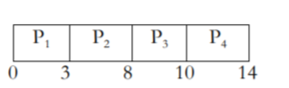
The waiting time for process
P1= 0, P2= 3, P3= 8, P4= 10
then the turnaround time for process
P1 = 0 + 3 = 3,
P2 = 3 + 5 = 8,
P3 = 8 + 2 = 10,
P4 = 10 + 4 =14.
Then average waiting time = (0 + 3 + 8 + 10)/4 = 21/4 = 5.25
Average turnaround time = (3 + 8 + 10 + 14)/4 = 35/4 = 8.75
The FCFS algorithm is non preemptive means once the CPU has been allocated to a process then the process keeps the CPU until the release the CPU either by terminating or requesting I/O.
2. Shortest Job First Scheduling (SJF) Algorithm:
This algorithm associates with each process if the CPU is available. This scheduling is also known as shortest next CPU burst, because the scheduling is done by examining the length of the next CPU burst of the process rather than its total length. Consider the following example:
| Process | CPU time |
|---|---|
| P1 | 3 |
| P2 | 5 |
| P3 | 2 |
| P4 | 4 |
Solution:According to the SJF the Gantt chart will be
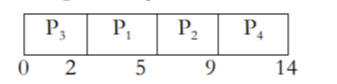
The waiting time for process P1 = 0, P2 = 2, P3 = 5, P4 = 9
then the turnaround time for process
P3 = 0 + 2 = 2,
P1 = 2 + 3 = 5,
P4 = 5 + 4 = 9,
P2 = 9 + 5 =14.
Then average waiting time = (0 + 2 + 5 + 9)/4 = 16/4 = 4
Average turnaround time = (2 + 5 + 9 + 14)/4 = 30/4 = 7.5
The SJF algorithm may be either preemptive or non preemptive algorithm. The preemptive SJF is also known as shortest remaining time first.
Consider the following example.
| Process | Arrival Time | CPU time |
|---|---|---|
| P1 | 0 | 8 |
| P2 | 1 | 4 |
| P3 | 2 | 9 |
| P4 | 3 | 5 |
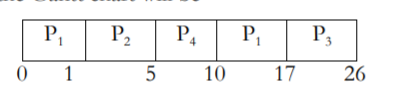
In this case the Gantt chart will be
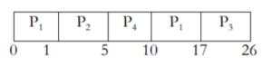
The waiting time for process
P1 = 10 – 1 = 9
P2 = 1 – 1 = 0
P3 = 17 – 2 = 15
P4 = 5 – 3 = 2
The average waiting time = (9 + 0 + 15 + 2)/4 = 26/4 = 6.5
3. Priority Scheduling Algorithm
In this scheduling a priority is associated with each process and the CPU is allocated to the process with the highest priority. Equal priority processes are scheduled in FCFS manner.
Consider the following example:
| Process | Arrival Time | CPU time |
|---|---|---|
| P1 | 10 | 3 |
| P2 | 1 | 1 |
| P3 | 2 | 3 |
| P4 | 1 | 4 |
| P5 | 5 | 2 |
According to the priority scheduling the Gantt chart will be
The waiting time for process
P1 = 6
P2 = 0
P3 = 16
P4 = 18
P4 = 1
The average waiting time = (0 + 1 + 6 + 16 + 18)/5 = 41/5 = 8.2
4. Round Robin Scheduling Algorithm
This type of algorithm is designed only for the time sharing system. It is similar to FCFS scheduling with preemption condition to switch between processes. A small unit of time called quantum time or time slice is used to switch between the processes. The average waiting time under the round robin policy is quiet long.
Consider the following example:
| Process | CPU time |
|---|---|
| P1 | 3 |
| P2 | 5 |
| P3 | 2 |
| P4 | 4 |
Time Slice = 1 millisecond
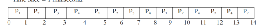
The waiting time for process
P1 = 0 + (4 – 1) + (8 – 5) = 0 + 3 + 3 = 6
P2 = 1 + (5 – 2) + (9 – 6) + (11 – 10) + (12 – 11) + (13 – 12) = 1 + 3 + 3 + 1 + 1 + 1 = 10
P3 = 2 + (6 – 3) = 2 + 3 = 5
P4 = 3 + (7 – 4) + (10 – 8) + (12 – 11) = 3 + 3 + 2 + 1 = 9
The average waiting time = (6 + 10 + 5 + 9)/4 = 7.5